Detecting Locations with NER

By Aaron Braunstein, Clare Jensen, and Kaitlyn Sisk

This page discusses the digital data collection tool Named Entity Recognition (NER) and its use in organizing the geographic information in runaway slave advertisements.

Rationale

In past analyses of runaway slave advertisements, the primary method utilized to collect data has been close reading, as illustrated in John Hope Franklin and Loren Schweninger’s book Runaway Slaves: Rebels on the Plantations. The authors chose fugitive slave advertisements as relatively credible sources since owners would have high incentives to provide accurate descriptions so their runaway(s) could easily be identified. They employed close reading to observe the nature of slavery on a personal level (Franklin and Scheninger, 295).

Our goal was to understand differences in location references within runaway slave ads across the Texas, Arkansas, and Mississippi corpora. After a close reading of the ads, we hypothesized that Texas ads were more self-referential than those of Arkansas and Mississippi. In addition, we noticed that Texas ads exclusively mentioned Mexico. Without digital tools to sift through the information, and with over 2500 advertisements in the corpora, we wouldn’t been able to feasibly collect the data to analyze these hypotheses. Thus, we needed an automatic way to compile comprehensive lists of state mentions in each of the three runaway ad corpora (Arkansas, Mississippi, and Texas).

Named Entity Recognition came to the rescue. Named Entity Recognition (NER) gave us the ability to extract the names of locations mentioned in each ad automatically. With the locations in hand, we needed a way to count, for each corpus, the number of ads that referenced a given state. Read on for a walkthrough of the entire process.

Methodology

For each corpus, we wanted to compute for each state and for Mexico the number of ads that “name-dropped” that location. To do that, we decided to utilize a combination of named entity recognition, via Stanford NER, and address lookup, via the geopy Python library using the GoogleV3 geocoder.

Please note that we do not discriminate between state reference types. That means, locations used in the context of where a slave was projected to run to count, locations used in the context of where a slave used to live count, even locations used in the context of where the sheriff’s dog live count. Any and all locations are valid locations for our analysis. Identifying just “ran from” and “ran to” locations is a much more complex task that we did not tackle.

Named Entity Recognition

Wikipedia defines named entity recognition succinctly:

Given a stream of text, determine which items in the text map to proper names, such as people or places, and what the type of each such name is (e.g. person, location, organization).

Stanford’s implementation of NER uses a Conditional Random Field (CRF) in order to label a string of text with entities. If you have taken statistics courses, you might be familiar with Hidden Markov Models, which are widely used in the realm of natural language processing for tasks like speech recognition and identifying part of speech of words in a sentence. CRF is very similar to that: the classifier used by NER is trained on a large data set containing a sequence of words in sentences, where each word is annotated with an entity category, if there is one. Then, using sliding windows that take into account words that come before and words that come after the tokens (words) in question, the program stochastically generates a state (label) for each word, whether that be “location,” “organization,” “person,” etc. Because it is probabilistic, there will always be errors, both false positives and false negatives. For a more technical overview of the differences of HMMs and CRFs, please read this blog post.

Generating a List of Referenced Locations in Each Ad

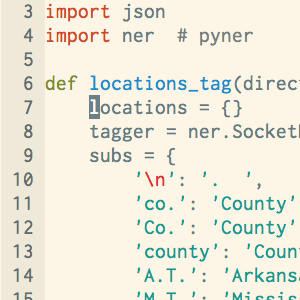
Our first task was to find all location names. As mentioned, we chose Stanford’s Named Entity Recognition software to use to identify locations in our corpora of runaway slave ads. We chose to write our entity tagger script in Python, and fortunately there is an interface called Pyner that hooks calls to the NER program.

Once we downloaded NER and cd’d to the directory, we started it with the following UNIX command. For an explanation of the arguments to the NER program, please read this short introduction to initializing NER for using Pyner. Note that we use the english.conll.4class classifier. It served our purposes, but if you want to train your own classifier, you can of course do that. The Wilkens Group at the University of Notre Dame has a good tutorial on training your own classifier if you are interested. They used NER on a 19th century American Fiction data set, and their tutorial outlines the advantages of training your own classifier.

java -mx1000m -cp stanford-ner.jar edu.stanford.nlp.ie.NERServer -loadClassifier classifiers/english.conll.4class.distsim.crf.ser.gz -port 8080 -outputFormat inlineXML

Then in Python, after installing Pyner, we initialized the tagger with the following command:

tagger = ner.SocketNER(host='localhost', port=8080)

Next, we called the get_entities method of the tagger, iteratively using each runaway slave ad in the corpus (a directory name) as the parameter. We checked if the LOCATION key existed in the entities dictionary (it also tags person, organization, etc), and if so, stored the LOCATION values in a locations dictionary that maps each filename to the detected locations:

for filename in os.listdir(directory):
    if filename.endswith(".txt"):
        with open(os.path.join(directory, filename), 'r') as f:
            text = f.read().decode("utf8")
            entities = tagger.get_entities(text)
            if 'LOCATION' in entities:
                locations[filename] = entities['LOCATION']

One problem that came up was that location tokens were as small as possible–usually at the word level. That means, if the text contained the phrase “Springfield, Virginia”, the locations list would usually separate entries for “Springfield” and “Virginia.” That behavior is not ideal since it can lead to ambiguity in the location names, and excess results. For example, there are dozens of towns named Springfield in the U.S. More on the ambiguity problem in a bit, but for now, our solution was a function that merges detected locations if they are situated within a certain threshold apart in the original text. We chose a maximum gap length of 2 between the tagged locations for them to be classified as an expression.

def merge_locations(locs, text):
    """Merges all words in locs list that are spaced at most two characters
    apart in text. (i.e. ", "). Assumes locs are in order in text.
    """
    idx = 0
    last_idx = len(locs) - 1
    merged = []
    while idx <= last_idx:
        loc = locs[idx]
        while not idx is last_idx:
            # "Trims" the text after looking at each location to prevent
            # indexing the wrong occurence of the location word if it
            # occurs multiple times in the text.
            gap, text, merge = gap_length(locs[idx], locs[idx+1], text)
            if gap <= 2:
                loc += merge
                idx += 1
            else:
                break
        merged.append(loc)
        idx += 1
    return merged
    
def gap_length(word1, word2, text):
    """Returns the number of characters after the end of word1 and
    before the start of word2 in text. Also returns the "trimmed"
    text with whitespace through word1's position and the
    merged words expression.
    """
    pos1, pos2 = text.index(word1), text.index(word2)
    pos1_e, pos2_e = pos1 + len(word1), pos2 + len(word2)
    gap = pos2 - pos1_e
    
    # Substitute characters already looked at with whitespace
    edited_text = chr(0)*pos1_e + text[pos1_e:]
    inter_text = text[pos1_e:pos2_e]
    return gap, edited_text, inter_text

Finally, we dumped the resulting filename -> locations dictionary as a JSON file. Click here for an example of our locations file for the Arkansas corpus.

with open(directory + '.json', 'w') as f:
    f.write(json.dumps(
                    locations,
                    indent=4,
                    separators=(',', ': ')
                    )
                )

If you would like to view the entire script or use it in your project, please visit this page. Note the script also does some preprocessing of the text specific to our data set to aid in the location detection.

Application

Now that we had a list of locations for each ad, we could tackle our original problem of calculating for each state the number of ads in each corpus that referenced that state.

The algorithm:

CountStateReferences

The above algorithm makes a few assumptions about the model governing the types of locations that appear in the text. Notice how first, we try to directly match the location to a known list of state names (e.g. “Arkansas”) and abbreviations (e.g. “AR” and “Ark.”). If it fails, we next try to look up an address for the location. We implemented this using the geopy library with the GoogleV3 geocoder. The github for the project contains some examples of doing geolocating and address lookup similar to this. Because NER often produces false positives–for example in our data, subscriber names often appeared in all caps and were inaccurately tagged as locations–we check that the result is an address in the region. We chose to make the assumption that true locations always either:

Include a state name in the merged location entity, or
Are a reference to a local or nearby location

This helps reduce the number of false positives (e.g. names of people) that are considered as state references, since Google Maps is very good at finding addresses for any input query, whether or not it’s an actual location. Also keep in mind that the probability that the address it chooses to return for non-location terms is in the nearby area (for example, Arkansas, Mississippi, Texas, Georgia, Tennessee, Louisiana, and Missouri) is low but of course non-negligible.

Also note that since we are storing the state abbreviations in a set, each ad will include each state in its mentions set at most once. Sets do not allow duplicate items, so the results reflect the number of ads referencing each state, instead of the number of times each state is referenced.

For comparison, we also implemented a different solution, using purely direct hits. This is functionally equivalent to just manually searching keywords (e.g. “Ark.”, “AK”, “Arkansas”) for each state in each corpus and tallying the results. If you want to minimize the number of false positives due to noise in the data, this is the way to go. However, it is very restrictive and requires a predefined list of keywords for each state. It is inflexible: for example, if we wanted to include “Canada” in our results, we would need to update the keywords list. And if there were keywords associated with real locations we didn’t think of (for example, misspellings of state names that the Google API could resolve but direct hits would miss), merely matching each location against that predefined list of keywords would miss them.

Conclusions

There are some limitations of NER that should be kept in mind. For one, it can sometimes tag items incorrectly. For example, we found that names of slaves or slave owners were sometimes tagged as locations, and places such as rivers could be tagged inaccurately as the location “Colorado” as opposed to being interpreted as “Colorado River.” These outliers can be cleaned up manually, but with a large corpus such as ours, it can be very time consuming. Even a well-written NER script will still make some mistakes, so cleaning up the data is a necessary step when using NER. That said, due to the nature of our project and the focus on the tool rather than the conclusions, we did not manually clean up our tagged locations. We also did not modify our final state counts in any way. Note how, for example, there are many hits for Washington. These are not true hits, but partial matches from “Washington County, Texas.” We left them in to illustrate a limitation of this method of counting state references.

A limitation of computing state counts algorithm is ambiguous place names, as previously mentioned with the Springfield example. Not to mention, state counts are affected by noise in the tagged locations data. To address this, in addition to the algorithm’s design, we could reduce the noise at the locations tagging level by being more strict about tagged location matches. Right now, we only ran the data with one classifier, but to reduce the number of false positives (at the risk of reducing true positives), we could run the data with multiple classifiers, and only take as true the tagged locations that were matched by every classifier. If that produces too little data, we could set a threshold such as 2/3 for the number of classifiers that have to match a given token.

Using NER with Google Fusion Tables

Google Fusion Tables, which merges together spreadsheets with geographic information, provides us a way to visualize the different results that NER can give. (This tutorial is helpful for learning how to use Google Fusion Tables).

The first map below for each state shows the results using only direct hits, i.e. locations that include a state name or state abbreviation in the word. The second map for each state shows the result using the CountStateReferences algorithm. Note how the numbers are larger in the algorithm maps. This is because the algorithm tries to resolve detected location terms that do not include the state name in them by querying the Google Maps API for an address associated with the location. If the address is in the nearby region (the South), we assume it is a real location and update the state counts accordingly.

Number of direct hit mentions of states in full Texas ad corpus, 1835-1860

Number of algorithm hit mentions of states in full Texas ad corpus, 1835-1860

Number of direct hit mentions of states in full Mississippi ad corpus, 1835-1860

Number of algorithm hit mentions of states in full Mississippi ad corpus, 1835-1860

Number of direct hit mentions of states in full Arkansas ad corpus, 1835-1860

Number of algorithm hit mentions of states in full Arkansas ad corpus, 1835-1860

When viewed in conjunction, the maps show that Texas runaway slave advertisements were indeed slightly more self-referential than advertisements in Arkansas and Mississippi, which supports our hypothesis. This could be due to the fact that Texas was a border land, so many runaway slaves were likely heading towards more remote areas, such as western Texas and Mexico, and not towards the rest of the Southern states. Texas is additionally the only state of the three to mention Mexico, but it does so fewer times than we were expecting. Arkansas is the least self-referential, which supports our earlier hypothesis outlined in the Palladio section that Arkansas was somewhat of a border land as well. The fact that about half of the total state references in the corpus are locations outside of Arkansas could be because Arkansas had more capture notices that advertised runaway slaves from other states.

DIGITAL HISTORY METHODS